前言
本文参考https://juejin.im/entry/5a1637f2f265da432528f6ef 的文章和 https://github.com/waleedka/traffic-signs-tensorflow 的源代码。
给定交通标志的图像,我们的模型应该能够知道它的类型。
首先我们要导入需要的库。
1 | import tensorflow as tf |
/home/song/anaconda3/lib/python3.6/site-packages/h5py/__init__.py:36: FutureWarning: Conversion of the second argument of issubdtype from `float` to `np.floating` is deprecated. In future, it will be treated as `np.float64 == np.dtype(float).type`.
  from ._conv import register_converters as _register_converters
1 加载数据和分析数据
1.1 加载数据
我们使用的是Belgian Traffic Sign Dataset。网址为http://btsd.ethz.ch/shareddata/
在这个网站可以下载到我们需要的数据集。你只需要下载BelgiumTS for Classification (cropped images):后面的两个数据集:
BelgiumTSC_Training (171.3MBytes)
BelgiumTSC_Testing (76.5MBytes)
我把这两个数据集分别放在了以下的路径:
/home/song/Downloads/BelgiumTSC_Training/Training
/home/song/Downloads/BelgiumTSC_Testing/Testing
Training目录包含具有从00000到00061的序列号的子目录。目录名称表示从0到61的标签,每个目录中的图像表示属于该标签的交通标志。 图像以不常见的.ppm格式保存,但幸运的是,这种格式在skimage库中得到了支持。
1 | def load_data(data_dir): |
1.2 分析数据
我们可以看一下我们的训练集中有多少图片和标签:
1 | print("Unique Labels: {0}\nTotal Images: {1}".format(len(set(labels)), len(images))) |
Unique Labels: 62
Total Images: 4575
这里的set很有意思,可以看一下这篇文章:http://www.voidcn.com/article/p-uekeyeby-hn.html
这里的set很有意思,可以看一下这篇文章:http://www.voidcn.com/article/p-uekeyeby-hn.html
在处理一系列数据时,如果需要剔除重复项,则通常采用set数据类型。本身labels里面是有很多重复的元素的,但set(labels)就剔除了重复项。可以通过print(labels)和print(set(labels))命令查看一下两者输出的有什么区别。
我们还可以通过画直方图来看一下数据的分布情况。
1 | plt.hist(labels,62) |
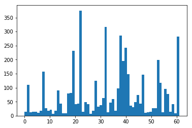
可以看出,该数据集中有的标签的分量比其它标签更重:标签 22、32、38 和 61 显然出类拔萃。这一点之后我们会更深入地了解。
1.3 可视化数据
1.3.1 热身
我们可以先随机地选取几个交通标志将其显示出来。我们还可以看一下图片的尺寸。我们还可以看一下图片的最小值和最大值,这是验证数据范围并及早发现错误的一个简单方法。其中的plt.axis(‘off’)是为了不在图片上显示坐标尺,大家可以注释掉这句话看看如果去掉有什么不一样。
1 | traffic_signs=[100,1050,3650,4000] |
shape: (292, 290, 3), min: 0, max: 255
shape: (132, 139, 3), min: 4, max: 255

shape: (146, 110, 3), min: 7, max: 255
shape: (110, 105, 3), min: 3, max: 255
大多数神经网络需要固定大小的输入,我们的网络也不例外。 但正如我们上面所看到的,我们的图像大小并不完全相同。 一种常见的方法是将图像裁剪并填充到选定的纵横比,但是我们必须确保在这个过程中我们不会切断部分交通标志。 这似乎需要进行手动操作! 我们其实有一个更简单的解决方案,即我们将图像大小调整为固定大小,并忽略由不同长宽比导致的失真。 这时,即使图片被压缩或拉伸了一点,我们也可以很容易地识别交通标志。我们用下面的命令将图片的尺寸调整为3232。
大多数神经网络需要固定大小的输入,我们的网络也不例外。 但正如我们上面所看到的,我们的图像大小并不完全相同。 一种常见的方法是将图像裁剪并填充到选定的纵横比,但是我们必须确保在这个过程中我们不会切断部分交通标志。 这似乎需要进行手动操作! 我们其实有一个更简单的解决方案,即我们将图像大小调整为固定大小,并忽略由不同长宽比导致的失真。 这时,即使图片被压缩或拉伸了一点,我们也可以很容易地识别交通标志。我们用下面的命令将图片的尺寸调整为3232。
1.3.2 重调图片的大小
1 | images32 = [transform.resize(image,(32,32)) for image in images] |
/home/song/.local/lib/python3.6/site-packages/skimage/transform/_warps.py:105: UserWarning: The default mode, 'constant', will be changed to 'reflect' in skimage 0.15.
  warn("The default mode, 'constant', will be changed to 'reflect' in "
/home/song/.local/lib/python3.6/site-packages/skimage/transform/_warps.py:110: UserWarning: Anti-aliasing will be enabled by default in skimage 0.15 to avoid aliasing artifacts when down-sampling images.
  warn("Anti-aliasing will be enabled by default in skimage 0.15 to "
重新运行上面随机显示交通标志的代码。
重新运行上面随机显示交通标志的代码。
1 | traffic_signs=[100,1050,3650,4000] |

shape: (32, 32, 3), min: 0.0, max: 1.0

shape: (32, 32, 3), min: 0.038373161764705975, max: 1.0

shape: (32, 32, 3), min: 0.05559895833333348, max: 1.0

shape: (32, 32, 3), min: 0.048665364583333495, max: 1.0
从上面的图和shape的值都能看出,图片的尺寸一样大了。最小值和最大值现在的范围在0和1.0之间,和我们未调整图片大小时的范围不同。
从上面的图和shape的值都能看出,图片的尺寸一样大了。最小值和最大值现在的范围在0和1.0之间,和我们未调整图片大小时的范围不同。
1.3.3 显示每一个标签下的第一张图片
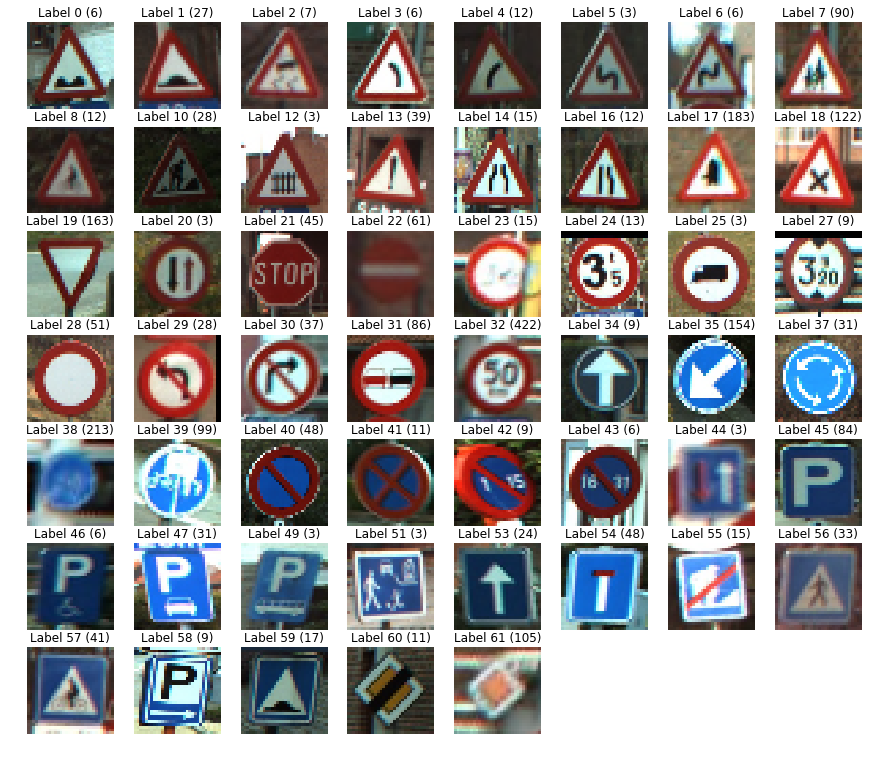
之前我们在直方图中看过62个标签的分布情况。现在我们尝试将每个标签下的第一张图片显示出来,另外还可以通过列表的count()方法来统计某个标签出现的次数,也就是能统计出有多少张图片对应该标签。我们可以定义一个函数,名为display_images_and_labels,你当然可以定义成别的名字,不过定义函数是为了之后可以方便地调用。以下分别显示出了未调整尺寸和已调整尺寸的交通标志图。
1 | def display_images_and_labels(images, labels): |
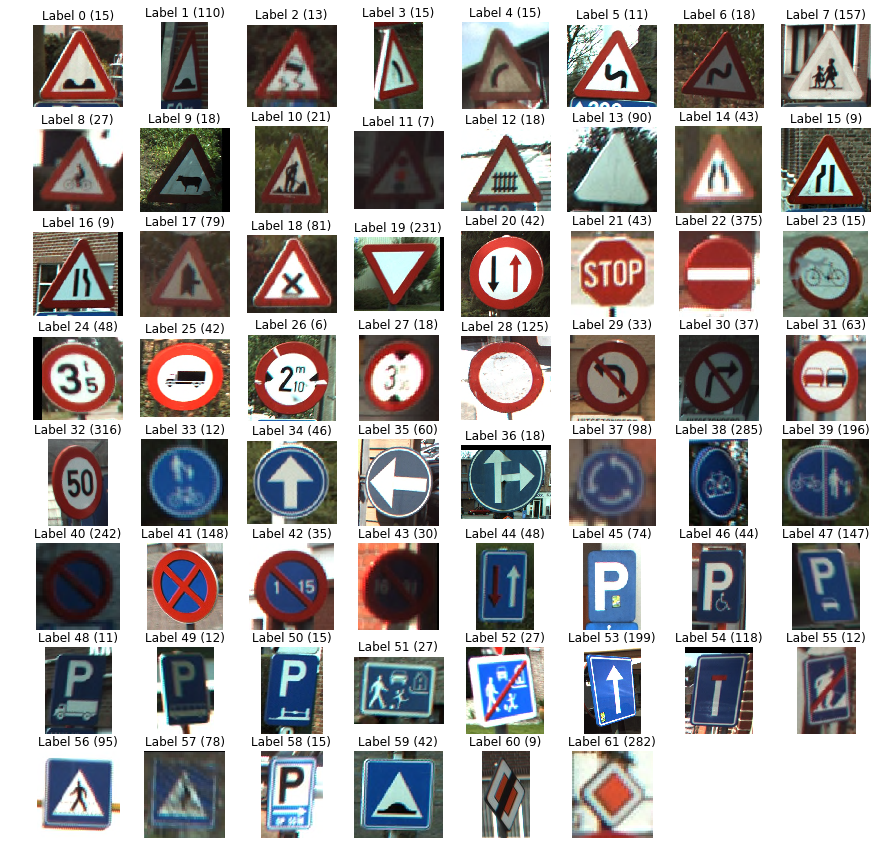
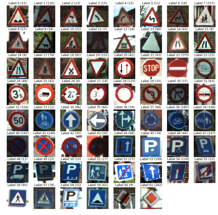
正如我们在直方图中看到的那样,具有标签 22、32、38 和 61 的交通标志要明显多得多。图中可以看到标签 22 有 375 个实例,标签 32 有 316 实例,标签 38 有 285 个实例,标签 61 有 282 个实例。
1.3.4 显示某一个标签下的交通标志
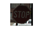
看过每个标签下的第一张图片之后,我们可以将某一个标签下的图片展开显示出来,看看这个标签下的是否是同一类交通标志。我们不需要把该标签下的所有图片都显示出来,可以只展示24张,你可以更改为其他的数字,显示更多或者更少。我们这里选择标签为21的看一下,在之前的图片中可以看到,label 21对应于stop标志。
1 | def display_label_images(images, label): |
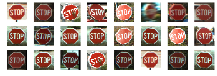
可以看出,label 21对应的前24张图片都是stop标志。不难推测,整个label 21对应的应都是stop标志。
2 构建深度网络
2.1 构建TensorFlow图并训练
首先,我们创建一个Graph对象。TensorFlow有一个默认的全局图,但是我们不建议使用它。设置全局变量通常太容易引入错误了,因此我们自己创建一个图。之后设置占位符来放图片和标签。注意这里参数x的维度是 [None, 32, 32, 3],这四个参数分别表示 [批量大小,高度,宽度,通道] (通常缩写为 NHWC)。我们定义了一个全连接层,并使用了relu激活函数进行非线性操作。我们通过argmax()函数找到logits最大值对应的索引,也就是预测的标签了。之后定义loss函数,并选择合适的优化算法。这里选择Adam算法,因为它的收敛速度比一般的梯度下降算法更快。这个时候我们只刚刚构建图,并且描述了输入。我们定义的变量,比如,loss和predicted_labels,它们都不包含具体的数值。它们是我们接下来要执行的操作的引用。我们要创建会话才能开始训练。我这里把循环次数设置为301,并且如果i是10的倍数,就打印loss的值。
1 | g = tf.Graph() |
images_flat:  Tensor("Flatten/flatten/Reshape:0", shape=(?, 3072), dtype=float32)
logits:  Tensor("fully_connected/Relu:0", shape=(?, 62), dtype=float32)
loss:  Tensor("Mean:0", shape=(), dtype=float32)
predicted_labels:  Tensor("ArgMax:0", shape=(?,), dtype=int64)
Loss:  4.181018
Loss:  3.0714655
Loss:  2.6622696
Loss:  2.4586942
Loss:  2.3419585
Loss:  2.2633858
Loss:  2.2044215
Loss:  2.157206
Loss:  2.1180305
Loss:  2.0847433
Loss:  2.0559382
Loss:  2.030667
Loss:  2.008251
Loss:  1.9882014
Loss:  1.9701369
Loss:  1.9537587
Loss:  1.938837
Loss:  1.9251733
Loss:  1.912607
Loss:  1.9010073
Loss:  1.8902632
Loss:  1.8802778
Loss:  1.8709714
Loss:  1.8622767
Loss:  1.8541412
Loss:  1.8465083
Loss:  1.8393359
Loss:  1.8325756
Loss:  1.8261962
Loss:  1.8201678
Loss:  1.8144621
2.2使用模型
2.2使用模型
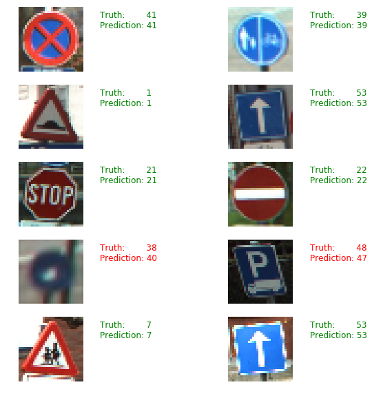
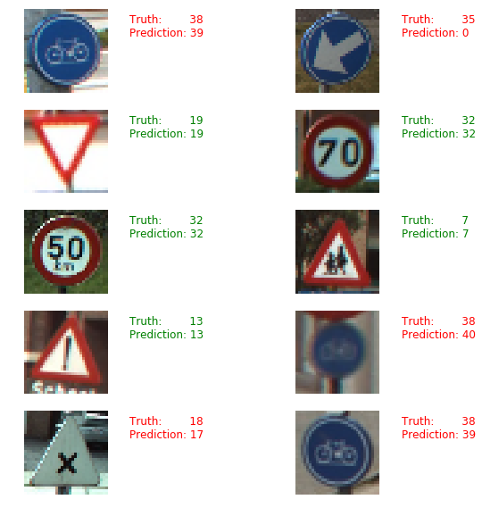
现在我们用sess.run()来使用我们训练好的模型,并随机取了训练集中的10个图片进行分类,并同时打印了真实的标签结果和预测结果。
1 | # Pick 10 random images |
[41, 39, 1, 53, 21, 22, 38, 48, 7, 53]
[41 39  1 53 21 22 40 47  7 53]
1 | ```python |
2.3评估模型
以上,我们的模型只在训练集上是可以正常运行的,但是它对于其他的未知数据集的泛化能力如何呢?我们可以在测试集当中进行评估。我们还可以计算一下准确率。
1 | test_images, test_labels = load_data(test_data_dir) |
/home/song/.local/lib/python3.6/site-packages/skimage/transform/_warps.py:105: UserWarning: The default mode, 'constant', will be changed to 'reflect' in skimage 0.15.
  warn("The default mode, 'constant', will be changed to 'reflect' in "
/home/song/.local/lib/python3.6/site-packages/skimage/transform/_warps.py:110: UserWarning: Anti-aliasing will be enabled by default in skimage 0.15 to avoid aliasing artifacts when down-sampling images.
  warn("Anti-aliasing will be enabled by default in skimage 0.15 to "


Accuracy: 0.5631
[38, 35, 19, 32, 32, 7, 13, 38, 18, 38]
[39  0 19 32 32  7 13 40 17 39]
2.4关闭会话
1 | sess.close() |
最后,记得关闭会话。